Simulating Inventory Policies with SimPy

Written in August 2025, when I built the simulator behind the inventory simulation demo. Rerun on 8 October 2026 with the same code: the tables below are from that rerun, and the bugs in What went wrong were found then.

Fixed reorder rules ignore variability, so they produce both overstock and stockouts at the same time. I wanted a small simulator that shows the cost of a reorder rule under random demand and random lead times, product by product, before trying to optimize anything.

The model

Each product follows exactly one policy: (r,Q), order a fixed quantity Q when the inventory position falls to r, or (s,S), order up to S. Customers arrive as a Poisson process, each one buys a random discrete amount, and every order arrives after an exponential lead time. A product either backorders unmet demand or loses it.

Every review period the loop is the same:

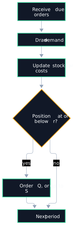
The inventory position is on hand plus outstanding orders. The cost per period is holding plus shortage plus ordering (a setup cost per order and a cost per unit), averaged over the horizon. The engine is SimPy, with NumPy and Python’s random module for the draws (both seeded together), behind a small FastAPI service.

What I ran

Two products from the demo’s defaults, 60 periods each, 50 seeded runs per reorder point:

Product	Policy	Demand	Lead time (mean)	Unmet demand
A	(s,S), S = 50	10 customers/period, 0.5, 1 or 1.5 units each	3 periods	backordered
B	(r,Q), Q = 15	8 customers/period, 1, 2 or 3 units each	2 periods	lost

Both use holding 1, shortage 5, setup 32 and unit cost 3.

Product A

r	Mean cost/period	SD	Min to max	Fill rate
10	96.4	25.6	61.0 to 190.9	0.62
20	87.8	18.3	63.4 to 144.6	0.66
30	79.4	14.4	59.4 to 131.1	0.75
40	79.1	8.5	66.4 to 101.1	0.84

Product B

r	Mean cost/period	SD	Min to max	Fill rate
10	84.0	4.1	72.6 to 93.2	0.37
20	88.0	3.9	77.7 to 96.9	0.60
30	91.7	3.8	80.7 to 99.2	0.73
40	94.9	3.5	83.5 to 102.8	0.78
50	99.2	3.2	89.4 to 109.3	0.84

(Product A’s fill rates are corrected; see What went wrong.)

What the numbers say

One run is not an answer. At r = 10, a single 60-period run of Product A costs anywhere from 61 to 191 per period. Any comparison of reorder points needs many runs, or the same random demand for both options.

Product B gets cheaper the less it sells. Its cost rises with r, and the cheapest rule serves only 37 percent of demand. That is the cost function talking, not inventory theory: there is no revenue in it. Serving one unit costs about 5.1 (unit cost 3, setup 32 / 15, plus holding), while losing it costs 5. An optimizer will happily learn to stop selling. To fix the model, add the lost margin to the shortage cost of lost-sales products, or require a minimum fill rate. I wrote about the same trap in testing a cost function before optimizing.

What went wrong

The fill rate was wrong for backordered products. A backorder stays in negative stock, and in every later period the whole backlog was counted again as new unmet demand. Product A’s fill rate came out as 0.002 at r = 10, and the optimizer’s copy of the engine reported negative fill rates for another product. The cost is fine (a backorder cost per unit per period is a valid choice); only the metric was broken. The fix is one line in the demand step:

self.unmet_demand += min(shortfall, demand)  # count only this period's unmet demand

With it, Product A’s fill rate is 0.62 to 0.84 instead of 0.002 to 0.74.

The API failed when history was off. run() returns the summary on its own when record_history is false, and a {"summary", "history"} pair when it is true, but the API always expects the pair. So POST /simulate with "record_history": false returns HTTP 400. Returning the same shape in both cases fixes it.

How to repeat this

The code is not public yet, but the API behind the demo is, and it gives the same numbers as my local runs (same seed, same result to the last decimal). One run of Product A at r = 20:

curl -s -X POST https://api-siminv.oploy.eu/simulate \
  -H "Content-Type: application/json" \
  -d '{"horizon": 60, "record_history": true, "random_seed": 1,
       "products": [{"name": "Product A", "reorder_point": 20, "reorder_up_to": 50,
         "demand_rate": 10, "demand_sizes": [0.5, 1, 1.5],
         "demand_probs": [0.3333333333, 0.3333333333, 0.3333333334],
         "lead_time_mean": 3}]}'

It returns "average_cost_per_period": 85.54166666666667 for seed 1.

1. Keep "record_history": true (see above).
2. Loop random_seed from 0 to 49 and average average_cost_per_period: that is one row of the tables.
3. Ignore the reported fill rate for backordered products until the fix above is deployed.

Or move the sliders in the demo. The next step, letting a genetic algorithm choose the reorder points, is in optimizing reorder points with a noisy simulator.