
Visualizing a Bi-Objective Repair-Shop Schedule
A schedule from my repair-shop scheduling work, with the model objectives, constraints, solution methods, and source code behind it.
First written in April 2025. The work behind it was published in the Decision Analytics Journal in 2026.
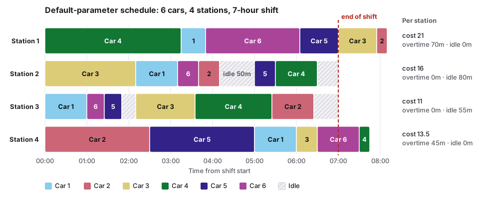
This chart is the schedule the web demo returns with its default parameters: six cars, four repair stations and a seven-hour shift, solved for the lowest idle and overtime cost. Each row is a station, each block is one car’s repair at that station, and its position shows the start and finish time. Hatched blocks are paid time with nothing to do, and anything right of the red line is overtime. The chart turns solver output into a sequence that an operator can inspect.
The optimization problem
The model is bi-objective. One objective reduces total flow time so jobs move through the system faster. The other reduces idle-resource and overtime cost. These objectives can conflict: compressing a schedule may improve completion time while creating expensive resource peaks, and a cheaper resource plan may delay jobs.
The constraints enforce feasible operation order, resource assignment, processing duration, and non-overlap. A valid solution must place every required operation on an eligible resource without allowing two operations to use the same capacity at the same time.
From mathematical model to comparable schedules
I implemented exact mixed-integer programming models and a modified NSGA-II search so I could compare solver-based and metaheuristic solutions. The multi-objective output is a set of non-dominated schedules rather than one unexplained answer. A decision maker can compare flow time with idle and overtime cost, then inspect the selected schedule in a chart like the one above.
Validation on real operational data produced about a 42 percent reduction in total flow time and a 47 percent reduction in idle and overtime costs relative to the comparison case reported in the study. Those figures belong to that dataset and experimental design. They are not universal performance claims.
Reuse the technical work
The public repository contains the official research code, including MATLAB, GAMS, OR-Tools, and FastAPI-related implementations. How the FastAPI version is deployed is in deploying FastAPI on Railway. If you adapt it, replace the operation times, eligible resources, precedence rules, capacity assumptions, and objective weights with your own system data. Then validate feasibility and objective units before comparing algorithms.
How to repeat this
The RepairShop-milp repository has three entry points:
Gams/Flow_time.gmsandGams/Idle_Over_time_cost.gms: the MILP, one file per objective (solved with CPLEX).MATLAB/Optimizer.m: the modified NSGA-II for larger instances.ORtools/Idle_Overtime.py: the CP-SAT version behind the web demo.
The fastest check needs no install: open the web demo, solve the sample day, and read the Gantt chart the same way as the one above. To compare with the paper, use Instance 1 from its Table 2 (28 cars, 49 repair procedures): the manual schedule had $469 of idle and overtime cost and 6,188 minutes of flow time; NSGA-II reached $267 and 3,925 minutes.
Read the peer-reviewed article. The code behind it is in the RepairShop-milp repository.