
Replacing a Slow Simulation with a Neural Network Metamodel
From my Master's thesis, published in 2025: an ANN metamodel against Kriging for simulations that take minutes per run, and where the comparison stops.
Written in May 2025. The work is from my Master’s thesis (2018); the article was accepted and published in 2025 after a long editorial process.
Some simulations take two to five minutes per run. That is too slow to call thousands of times inside an optimizer, but not slow enough to justify building a metamodel up front and trusting it blindly. Inventory models are a typical case (I wrote about a SimPy inventory simulation separately). The paper calls these semi-expensive problems, and asks which surrogate to use for them: an artificial neural network (ANN) or Kriging.
The method
The algorithm (ANN-SMB, a semi-metamodel-based method) works in two phases. This is the flow in main_core_ANN.m:
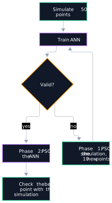
- Start: the corners of the search box plus a maximin Latin hypercube, 50 points in total, each simulated.
- Phase 1 explores with the real simulation: a particle swarm step adds 10 new simulated points per round, and the ANN is retrained, for at most three rounds or until the ANN passes validation (leave-one-out cross-validation with a studentized prediction error).
- Phase 2 exploits: the swarm searches the trained ANN instead of the simulation, and only the final point is simulated again.
- The ANN is a feed-forward network with one tan-sigmoid hidden layer (15 neurons in the code) and a linear output. The swarm is the paper’s spatial-hole PSO variant (SH-PSO).
The same framework with Kriging in place of the ANN is the comparison.
Results
On an (s,S) inventory model:
| Metric | ANN-SMB | Kriging-SMB |
|---|---|---|
| Average objective value | 595.28 | 603.71 |
| Standard deviation | 10.61 | 14.99 |
| Function evaluations | 262.5 | 264 |
On five analytical test functions, the ANN version was better on Sphere, Griewank, Schaffer F6 and Rosenbrock, and Kriging on Rastrigin, with 5 to 10 percent fewer function evaluations for the ANN.
What this does and does not show
The difference on the inventory model is not statistically significant (p = 0.913): solution quality is equivalent, and the ANN’s advantage is a smaller spread and slightly fewer evaluations. The tests go up to three decision variables, on continuous problems with low noise, and the result is sensitive to the number of hidden neurons (about 6 percent).
That boundary matters. When I later optimized reorder points for five products with a GA, the problem was discrete, five-dimensional and very noisy: exactly the case this paper does not cover.
What went wrong
The README lists the wrong parameters. It says to tune idp, r, m, h and epsilon in main_core_ANN.m; those names do not appear there. The real settings are at the top of the file (see below).
How to repeat this
You need MATLAB 8.4 or later with the Statistics and Machine Learning Toolbox.
% clone https://github.com/Mbehbahani/ANN-SMB-SemiExpSimOpt, then in MATLAB:
cd Main
main_core_ANN
- It starts on the Griewank test function,
f=@griewank, with bounds -8 to 8 in two dimensions. - For the inventory model, switch to the commented lines
f=@operationfunwithLower_Bound=[450,750]andUpper_Bound=[750,1050]. Num_o_Design_points=50sets the first design, andNum_o_Samples=1sets the replications per point.- Other test functions (
rosenbrock.m,rastr.m,schaffer2.m,funksphere.m) are in the same folder.
The article: An artificial neural network metamodel to solve semi-expensive simulation optimization problems: a comparative study, Journal of Industrial Engineering, 2025.